Nicer scatter plots in GGgally ggpairs-ggduo

GGally is an extension of ggplot2. I use it mainly as a replacement/refinement of pairs in base R.

Here, I want to replace the default scatter plot used to compare 2 continuous variables with something nicer, especially adapted to plotting large number of points.

Load the library and some RNA-seq data:

library(GGally)
library(airway)
data(airway)

The airway dataset contains data for 4 cell lines treated or not with dexamethasone:

colData(airway)[,1:3]

	SampleName	cell	dex
SRR1039508	GSM1275862	N61311	untrt
SRR1039509	GSM1275863	N61311	trt
SRR1039512	GSM1275866	N052611	untrt
SRR1039513	GSM1275867	N052611	trt
SRR1039516	GSM1275870	N080611	untrt
SRR1039517	GSM1275871	N080611	trt
SRR1039520	GSM1275874	N061011	untrt
SRR1039521	GSM1275875	N061011	trt

Let’s keep a fraction of the data for simplicity

df <- as.data.frame(assays(airway)$counts[,1:4]) #first 4 columns
df <- df[rowSums(df)>4,] #keep genes with some counts
set.seed(123)
df <- df[sample.int(nrow(df),1e3),] #random 1K genes

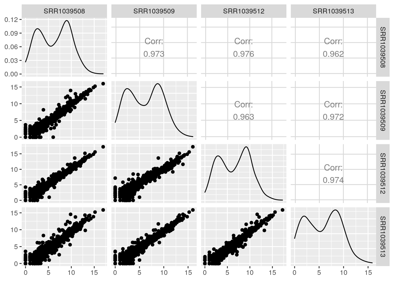
default behavior of GGally::ggpair:

GGally::ggpairs(log2(df+1))

Here is a better function to make the scatterplots in the lower triangle. It is largely based on this blog post and implements:

• viridis coloring of points based on expression level (practically based on effect size captured by the first principal component). I added some code to get consistent coloring even if orientation of the first PC differs between pairs of columns.
• alpha based on inverse of 2D density, i.e. low alpha when there are lots of points and higher when points are more scattered

Also, the use of GGally:eval_data_col is described here:

GGscatterPlot <- function(data, mapping, ..., 
                        method = "spearman") {

#Get correlation coefficient
    x <- GGally::eval_data_col(data, mapping$x)
    y <- GGally::eval_data_col(data, mapping$y)

    cor <- cor(x, y, method = method)
#Assemble data frame
    df <- data.frame(x = x, y = y)
# PCA
    nonNull <- x!=0 & y!=0
    dfpc <- prcomp(~x+y, df[nonNull,])
    df$cols <- predict(dfpc, df)[,1]
# Define the direction of color range based on PC1 orientation:
    dfsum <- x+y
    colDirection <- ifelse(dfsum[which.max(df$cols)] < 
                               dfsum[which.min(df$cols)],
                           1,
                           -1)
#Get 2D density for alpha
    dens2D <- MASS::kde2d(df$x, df$y)
    df$density <- fields::interp.surface(dens2D , 
                                         df[,c("x", "y")])

if (any(df$density==0)) {
    mini2D = min(df$density[df$density!=0]) #smallest non zero value
    df$density[df$density==0] <- mini2D
}
#Prepare plot
    pp <- ggplot(df, aes(x=x, y=y, color = cols, alpha = 1/density)) +
                ggplot2::geom_point(shape=16, show.legend = FALSE) +
                ggplot2::scale_color_viridis_c(direction = colDirection) +
#                scale_color_gradient(low = "#0091ff", high = "#f0650e") +
                ggplot2::scale_alpha(range = c(.05, .6)) +
                ggplot2::geom_abline(intercept = 0, slope = 1, col="darkred") +
                ggplot2::geom_label(
                        data = data.frame(
                                        xlabel = min(x, na.rm = TRUE),
                                        ylabel = max(y, na.rm = TRUE),
                                        lab = round(cor, digits = 3)),
                        mapping = ggplot2::aes(x = xlabel, 
                                               y = ylabel, 
                                               label = lab),
                        hjust = 0, vjust = 1,
                        size = 3, fontface = "bold",
                        inherit.aes = FALSE # do not inherit anything from the ...
                        ) +
                theme_minimal()

return(pp)
}

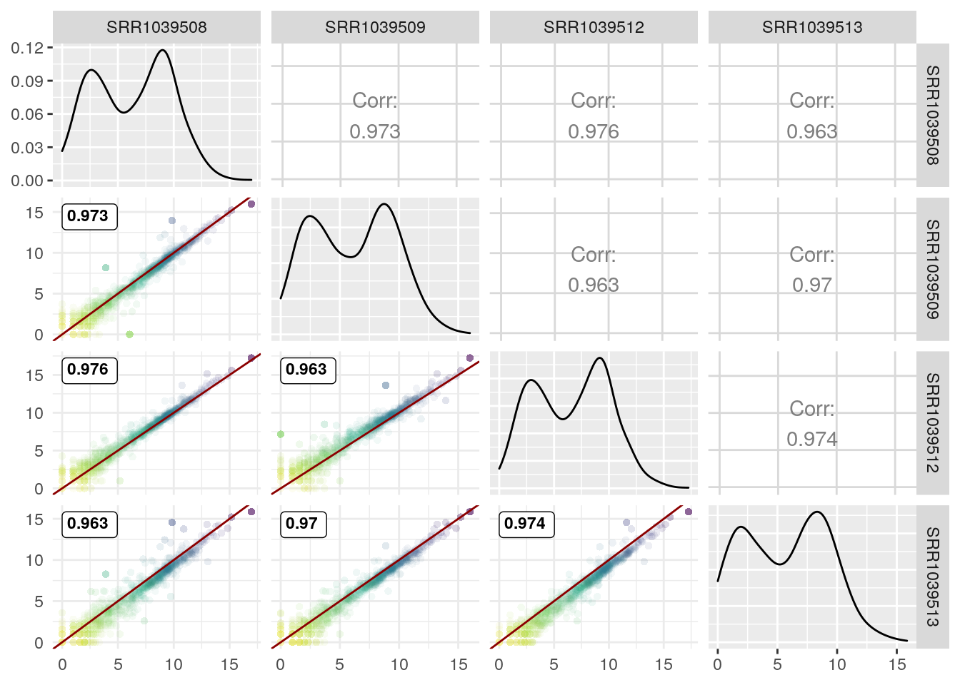
Now use in ggpairs (adjust correlation method to be consistent with defaults in GGscatterPlot):

GGally::ggpairs(log2(df+1),
                1:4,
                lower = list(continuous = GGscatterPlot),
                upper = list(continuous = wrap("cor", method= "spearman")))

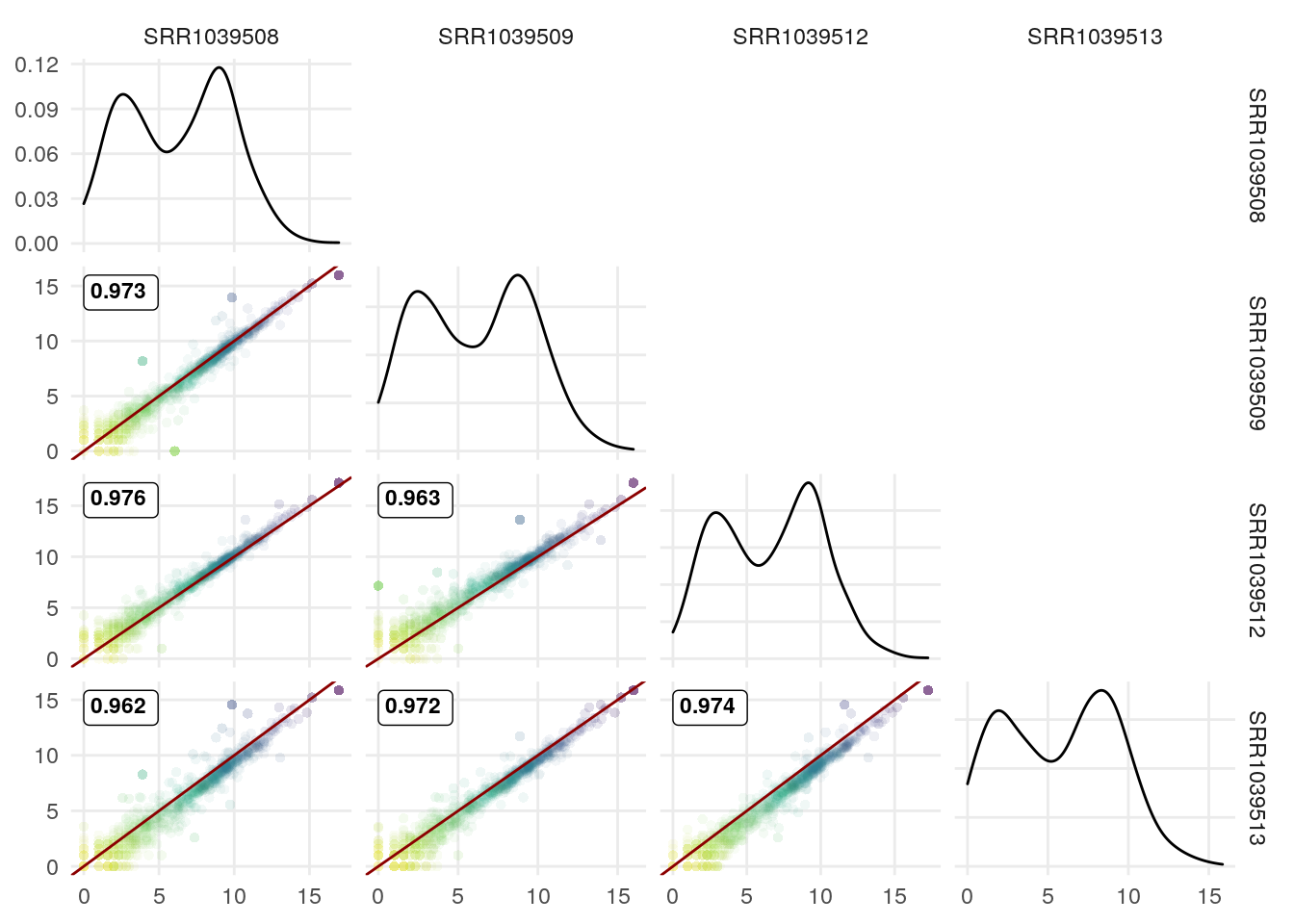
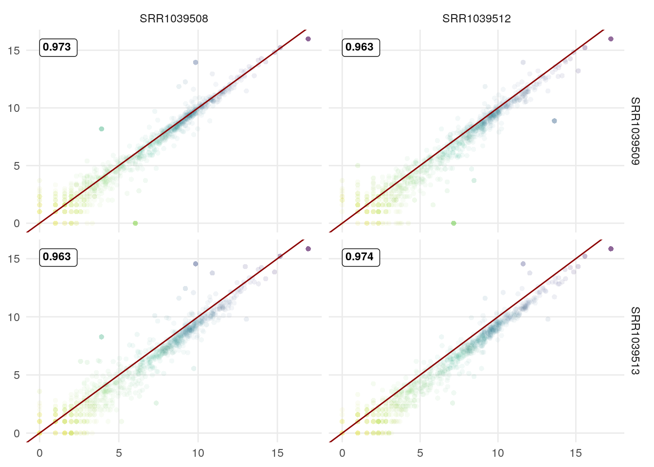
Now with Pearson correlation coefficient (and removing the correlation coefficient in the upper triangle since we already have them in the lower triangle):

GGally::ggpairs(log2(df+1),
                1:4,
                lower = list(continuous = wrap(GGscatterPlot, method="pearson")),
                upper = "blank") +
    theme_minimal() +
    theme(panel.grid.minor = element_blank())

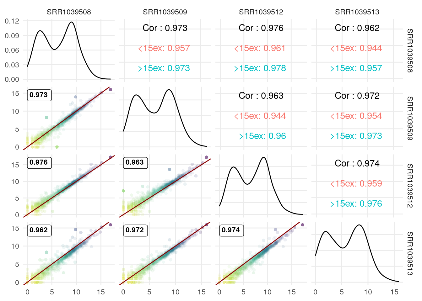
We can use the upper triangle to plot other info since the scatter plots include the correlation coefficient.
I illustrate it here with the correlation coefficient for genes with >15 exons vs those with <15 exons:

exonNumber <- elementNROWS(rowRanges(airway[rownames(df),]))
df$MoreThan15Exons <- ifelse(exonNumber>15,
                             ">15ex", "<15ex")
df[,1:4] <- log2(df[,1:4]+1)

GGally::ggpairs(df,
                1:4,
        lower = list(continuous = wrap(GGscatterPlot, method="pearson")),
        upper = list(continuous = wrap(ggally_cor, alignPercent = 0.8), 
                     mapping = ggplot2::aes(color = MoreThan15Exons))) +
    theme_minimal() +
    theme(panel.grid.minor = element_blank())

The GGscatterPlot function can also be used with GGally::ggduo to study the link between 2 sets of columns/samples. Here an example comparing control vs DEX samples:

GGally::ggduo(df,
              c(1,3), 
              c(2,4),
              types = list(continuous = GGscatterPlot)) +
    theme_minimal() +
    theme(panel.grid.minor = element_blank())